3 types of models are common in system identification: the black-box model, grey-box model, and user-defined model.
The black-box model assumes that systems are unknown and all model parameters are adjustable without considering the physical background. You cannot adjust all the parameters arbitrarily.
The grey-box model assumes that part of the information about the underlying dynamics or some of the physical parameters are known and the model parameters might have some constraints.
The user-define model assumes that commonly used parametric models cannot represent the model you want to estimate. You can define your special system model by using a template with a predefined input-output interface.
1. Black-box Model
A variety of parametric model structures are available to assist in modeling an unknown system. Parametric models describe systems in terms of differential equations and transfer functions. These models provide insight into the system physics and compact model structures. It is often beneficial to test a number of structures to determine the best one. A parametric model structure is also known as a black-box model, which defines either a continuous-time system or a discrete-time system.
General-linear model
Generally, you can describe a system using the following equation, which is known as the general-linear polynomial model or the general-linear model.
u(n) and y(n) are the input and output of the system respectively.
e(n) is zero-mean white noise, or the disturbance of the system.
is the transfer function of the deterministic part of the system.
is the transfer function of the stochastic part of the system.
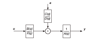
The general-linear model structure, shown in Figure 1, provides flexibility for both the system dynamics and stochastic dynamics. However, a nonlinear optimization method computes the estimation of the general-linear model. This method requires intensive computation with no guarantee of global convergence.
Figure 1 General-Linear Model Structure
Simpler models that are a subset of the General Linear model structure are possible. By setting one or more of A(q), B(q), C(q) or D(q) polynomials equal to 1 you can create these simpler models such as AR, ARX, ARMAX, Box-Jenkins, and output-error structures. Each of these methods has their own advantages and disadvantages and is commonly used in real-world applications.
For any particular problem the choice of the model structure to use depends on the dynamics and the noise characteristics of the system. Using a model with more freedom or parameters is not always better as it can result in the modeling of nonexistent dynamics and noise characteristics. This is where physical insight into a system is helpful.
AR Model
The AR model structure is a process model used in the generation of models where outputs are only dependent on previous outputs. No system inputs or disturbances are used in the modeling. This is a very simple model that is limited in the class of problems it can solve. Strictly speaking this means that the AR model structure is the model for a signal, not a system. Time series analyses, such as linear prediction coding commonly use the AR model.
Figure 2 AR Model Structure
ARX Model
The ARX model, shown in Figure 3, is the simplest model incorporating the stimulus signal. The estimation of the ARX model is the most efficient of the polynomial estimation methods because it is the result of solving linear regression equations in analytic form. Moreover, the solution is unique. In other words, the solution always satisfies the global minimum of the loss function. The ARX model therefore is preferable, especially when the model order is high.
The disadvantage of the ARX model is that disturbances are part of the system dynamics. The transfer function of the deterministic part G(q–1, è) of the system and the transfer function of the stochastic part H(q–1, è) of the system have the same set of poles. This coupling can be unrealistic. The system dynamics and stochastic dynamics of the system do not share the same set of poles all the time. However, you can reduce this disadvantage if you have a good signal-to-noise ratio.
When the disturbance e(n) of the system is not white noise, the coupling between the deterministic and stochastic dynamics can bias the estimation of the ARX model. Set the model order higher than the actual model order to minimize the equation error, especially when the signal-to-noise ratio is low. However, increasing the model order can change some dynamic characteristics of the model, such as the stability of the model.
Figure 3 ARX Model Structure
ARMAX Model
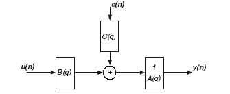
Unlike the ARX model, the ARMAX model structure includes disturbance dynamics. ARMAX models are useful when you have dominating disturbances that enter early in the process, such as at the input. For example, a wind gust affecting an aircraft is a dominating disturbance early in the process. The ARMAX model has more flexibility in the handling of disturbance modeling than the ARX model.
Figure 4 ARMAX Model Structure
Box-Jenkins Model
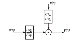
The Box-Jenkins (BJ) structure provides a complete model with disturbance properties modeled separately from system dynamics.
Figure 5 Box-Jenkins Model Structure
The Box-Jenkins model is useful when you have disturbances that enter late in the process. For example, measurement noise on the output is a disturbance late in the process.
Output-Error Model
The Output-Error (OE) model structure describes the system dynamics separately. No parameters are used for modeling the disturbance characteristics.
Figure 6 OE Model Structure
Transfer function Model
For stochastic control, the above general-linear polynomial models are commonly used because these models separately describe the deterministic and stochastic parts of a system. However, in classical control engineering, the deterministic part of the system is more important than the stochastic part. Transfer function models are commonly used to describe only the deterministic part of the system. Transfer function models can describe both continuous-time and discrete-time systems.
The following equations describe a continuous-time and discrete-time transfer function model, respectively.
y(t) = G(s)u(t)
y(k) = G(z)u(k) + e(k)
y(t) and y(k) are the system outputs. G(s) and G(z) is the transfer function between the stimulus and the response. u(t) and u(k) are the system inputs.
Use transfer function model structure to represent single-input and single-output (SISO) physical systems or multiple-input and single-output (MISO) physical systems. For more complicated multiple-input and multiple-output (MIMO) physical systems, use the state-space model structure.
State-Space Model
The previous classical parametric system identification methods minimize a performance function which is based on the sum of squared errors. These methods work well in many cases. However, for complex systems characterized by being of high order i.e. having many parameters, with several inputs and outputs, and having a large number of measurements, the classical methods can suffer from several problems. They can experience many local minima in the performance function and thereby a lack of convergence to global minima. The user will need to specify complicated parameterization of system orders and delays. They also may suffer potential problems with numerical instability and excessive computation time to execute the iterative numerical minimization methods needed. In addition, modern control methods require a state-space model of the system. For cases such as these the State-Space (SS) identification method is the appropriate model structure.
The following equations describe a state-space model.
x(n) is the state vector, y(n) is the system output, u(n) the system input and e(n) is the stochastic error. A, B, C, D, and K are the system matrices. The dimension of the state vector x(n) is the only setting you need to provide for the state-space model.
In general, the state-space model provides a more complete representation of the system, especially for MIMO systems, than polynomial models because the state-space model is similar to a first principle model. The identification procedure does not involve nonlinear optimization so the estimation reaches a solution regardless of the initial guess. Moreover, the parameter settings for the state-space model are simpler than polynomial models. You need to select only the order, or the number of states, of the model. The order can come from prior knowledge of the system. You also can determine the order by analyzing the singular values of the information matrix.
For MIMO systems, when the model order is high, use an ARX model because the algorithm involved in the ARX model estimation is fast and efficient when the number of data points is very large. The state-space model estimation with a large number of data points is slow and requires a large amount of memory. If you must use a state-space model, for example in modern control methods, reduce the sampling rate of the signal in case the sampling rate is unnecessarily high.
The other polynomial models, including the ARMAX, output-error, Box-Jenkins, and general-linear models, involve iterative, nonlinear optimization in the identification procedure. They require excessive computation time, and the minimization can get stuck at a false local minimum, especially when the order is high and the signal-to-noise ratio is low. However, you can use these models when the stochastic dynamics are important because they provide more flexibility for the stochastic dynamics.
2. Grey-box Model
In some circumstances, you have already obtained part of the information about the underlying dynamics or some of the physical parameters of the system. You can select the grey box model to specify these partially known physical parameters or some constraints. Then, you can estimate remaining unknown parameters with partially known model estimation methods. In the LabVIEW System Identification toolkit, two grey-box models are provided for you to represent the system, partially known state-space model and partially known transfer function model.
You can use partially known state-space model to describe physical systems in a continuous-time or discrete-time form with symbolic variables rather than numerical values. The physical system can be a SISO, MISO, or MIMO system. You can set a constant value or constraints (initial guesses and upper and lower limits) on each symbolic variable with prior knowledge.
For a simpler SISO physical system, you can also use the partially known transfer function model to describe the physical system in continuous-time form. You can apply the prior knowledge you have about the system’s physically meaningful parameters using the static gain, delay, time constant, natural frequency, and damping ratio inputs.
Grey-box model identification involves optimization process to minimize the difference between the estimated output and the measured real output> Finding the global optimum depends on the limit range you set and the initial values. To decrease the estimation time, you can set a narrow limit range and reasonable initial parameters.
3. User defined Model
Sometimes, you may find the parametric model and grey-box model cannot represent the physical system you want to estimate, especially when the physical system contains some non-linear factors.
Sources:
http://www.ni.com/white-paper/4028/en/


