While seat for a position as Assistant Research Officer, one of the most interesting but quit difficult for me to catch up in excel is VLOOKUP FUNCTION.
For now, i want to share information about it.
Use VLOOKUP when you need to find things in a table or a range by row. For example, look up find an employee name based on their employee ID.
In its simplest form, the VLOOKUP function says:
=VLOOKUP(What you want to look up, where you want to look for it, the column number in the range containing the value to return, return an Approximate or Exact match – indicated as 1/TRUE, or 0/FALSE).
How to get started
There are four pieces of information that you will need in order to build the VLOOKUP syntax:
The value you want to look up, also called the lookup value.
The range where the lookup value is located. Remember that the lookup value should always be in the first column in the range for VLOOKUP to work correctly. For example, if your lookup value is in cell C2 then your range should start with C.
The column number in the range that contains the return value. For example, if you specify B2:D11 as the range, you should count B as the first column, C as the second, and so on.
Optionally, you can specify TRUE if you want an approximate match or FALSE if you want an exact match of the return value. If you don’t specify anything, the default value will always be TRUE or approximate match.
Now put all of the above together as follows:
=VLOOKUP(lookup value, range containing the lookup value, the column number in the range containing the return value, Approximate match (TRUE) or Exact match (FALSE)).
Examples
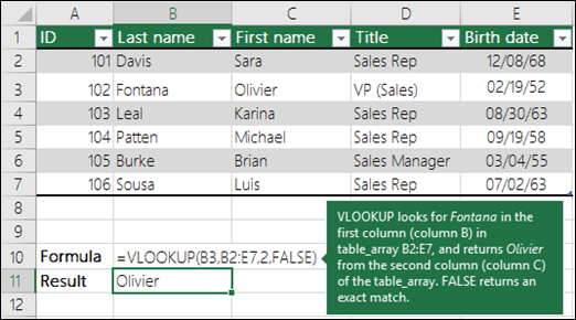
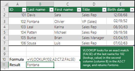
Here are a few examples of VLOOKUP:
Example 1

Example 2

Thank you. Source from : https://support.microsoft.com/en-us/office/vlookup-function-0bbc8083-26fe-4963-8ab8-93a18ad188a1

