Saint Venant Kinematic Wave Equations
Saint Venant equations are time dependent partial differential equations which describe the distribution of flow as a function of distance x along the channel and time t. The equations were first derived by Barre de Saint-Venant in 1871 (Vieux et.al., 1990). The equations were derived by considering the two conservation laws which are the conservation of mass and the conservation of momentum. The derivations of the equations from Reynolds transport theorem have been detailed in Chow et al. (1988) which are given herein in Appendix A. The final forms of the partial differential equations are given as follows.
Equation of Mass
∂A/dt+∂Q/∂x=q(x)
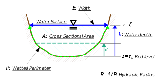
where A is the cross-sectional area of the flow, Q is the flow rate and q (x) is the forcing term (i.e. precipitation, lateral flow).
Equation of Momentum
1/A ∂Q/∂t+1/A ∂/∂x (Q^2/A)+g ∂y/∂x-g(S_o-S_f )=0
where S_0 is the bed slope and S_f is the frictional slope, whilst y and g are the depth of water and gravitational pull, respectively. The complete form of Eq. (2) is termed as full dynamics equation. If the first two terms on the left hand side of the equation are omitted, we then obtain diffusive equation.
However, Eq. (2) can be further approximated when it is assumed that S_o=S_f. This is known as the kinematics wave assumption (Vieux, 1988; Singh, 2003). This condition can be equivalently treated in Manning form as
A=αQ^β
where
α = (ηP^(2/3)/(1.49√(S_o )))^0.6
η = Manning roughness coefficient
P = wetted perimeter
S_o = bed slope
β = 0.6
Eq. (1) and (3) are the Saint Venant Kinematic Wave equations. By combining Eq. (1) and Eq. (3), the following equation can be obtained.
∂Q/∂t+1/αβ Q^((1-β) ) ∂Q/∂x=q
By discretizing (4) in time by forward-difference, we obtain
(Q^(t+1)-Q^t)/∆t+1/αβ Q^((1-β),t+1) (∂Q^(t+1))/∂x=q^(t+1)
where t+1 and t refers to present and previous time-step, respectively. Rearranging gives
Q^(t+1)+∆t/αβ Q^((1-β),t+1) (∂Q^(t+1))/∂x-Q^t=q^(t+1)