By Shahabuddin Amerudin
Introduction
In the realm of data analysis, regression analysis stands as a powerful tool that facilitates the exploration, understanding, and prediction of spatial relationships. By unraveling the intricate connections between variables, it provides insights into the factors driving observed spatial patterns. In this article, we delve into the fascinating world of regression analysis, focusing on its predictive applications through two distinct examples: the prediction of human deaths and the analysis of grave demand.
Regression analysis forms the cornerstone of modern statistical analysis, enabling us to move beyond mere correlation and into the realm of causation. As we journey through the depths of this method, we will explore its various techniques, from Ordinary Least Squares (OLS) to Geographically Weighted Regression (GWR), each contributing to our understanding of spatial phenomena. Join us as we uncover the mechanics, applications, and nuances of regression analysis, using human mortality and the demand for graves as our lenses into this dynamic field.
Among the array of regression techniques, Ordinary Least Squares (OLS) stands as the foundational technique, serving as the starting point for spatial regression analyses. OLS constructs a comprehensive model for the variable under scrutiny, such as the prediction of human deaths or the demand for graves, resulting in a single regression equation encapsulating that process.
Geographically Weighted Regression (GWR) is another influential spatial regression technique, finding increased adoption in geography and other fields. GWR generates localized models for the variable in focus. It involves fitting separate regression equations to each individual data point, capturing unique relationships within the immediate context. When employed effectively, these methods provide robust statistical tools for investigating and estimating linear relationships.
The nature of linear relationships is often either positive or negative. For instance, when local death rates rise with an increase in air pollution levels, it indicates a positive correlation. Similarly, if the demand for graves decreases as the population density rises, this signifies a negative relationship. Fig. 1 illustrates these positive, negative, and neutral relationships between variables.
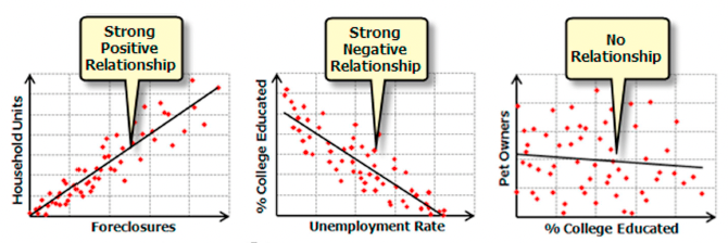
While correlation analysis gauges the strength of relationships between two variables, regression analysis delves deeper, aiming to quantify the extent to which one or more variables potentially contribute to positive or negative changes in another.
Unveiling Ordinary Least Squares (OLS)
Consider the equation depicted in Fig. 2, where the dependent variable (y) embodies the process being predicted or understood, such as the prediction of human deaths or the estimation of grave demand. In this equation, the dependent variable takes its place on the left side of the equation. The process of regression begins with a set of known y values, which are used to construct and calibrate the regression model. These known y values are often referred to as observed values.
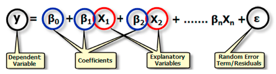
Independent/explanatory variables (x) are the driving forces behind modeling or predicting the values of the dependent variable. In the regression equation, these variables are positioned on the right side of the equation and are termed explanatory variables. The dependent variable responds to changes in these explanatory variables. For instance, predicting the demand for graves might involve variables such as population growth, cultural practices, urbanization levels, and mortality rates.
Regression coefficients (β) are calculated by the regression tool, representing the strength and direction of the relationship between each explanatory variable and the dependent variable. A positive relationship between grave demand and population growth, for instance, results in positive coefficients. Conversely, negative relationships yield negative coefficients. Strong relationships are reflected in large coefficients, while weak relationships manifest as coefficients closer to zero. The regression intercept (β0) signifies the expected value of the dependent variable when all independent variables are zero.
P-values indicate the probability that the coefficients for each independent variable are significantly different from zero. Small P-values indicate that a coefficient significantly contributes to the model, while coefficients near zero indicate minimal predictive impact unless supported by strong theoretical reasoning.
R2/R-Squared and Adjusted R-Squared gauge model performance. R-squared values range from 0 to 100%, with a value of 1.0 indicating a perfect fit. Adjusted R-Squared considers model complexity. Residuals measure the unexplained portion of the dependent variable.
Constructing a regression model entails iteratively selecting effective independent variables, utilising the regression tool to identify predictive variables, and refining the model for the optimal fit.
Navigating Geographically Weighted Regression (GWR)
Geographically Weighted Regression (GWR) offers a localized variant of linear regression, creating distinct equations for each data point by incorporating dependent and explanatory variables within a defined bandwidth. GWR’s efficacy hinges on user-defined parameters such as Kernel type, Bandwidth method, Distance, and Number of Neighbors.
For optimal results, GWR is most suited for datasets with numerous data points and is less effective for smaller datasets or multipoint data. Its outputs encompass a summary report, an Output feature class, and a diagnostic table. GWR is particularly useful when dealing with spatially varying relationships.
Practical Applications of Regression Analysis
Regression analysis finds application in diverse scenarios. For instance, it aids in modeling the prediction of human deaths to identify high-risk regions and comprehend the contributing factors. Analyzing property loss due to fatalities as influenced by factors like medical services access, response times, and population density is another application. In the realm of urban planning, regression helps dissect the demand for graves in relation to population growth, cultural dynamics, and mortality patterns.
Furthermore, regression analysis offers a means to test hypotheses. Investigating the correlation between urban development and grave demand, or exploring the relationship between healthcare access and human deaths, provides valuable insights. The tool also serves as a predictive instrument, helping anticipate trends in mortality rates or estimating the future demand for graves in regions without sufficient data.
In situations where interpolation falls short due to limited data, regression analysis provides a robust alternative, enabling prediction by modeling various phenomena.
Ultimately, regression analysis empowers researchers to uncover intricate relationships and harness predictive capabilities across a spectrum of scenarios, shedding light on the dynamics of human deaths and the demand for graves.
Conclusion
In the realm of data analysis, the power of regression analysis shines through as a beacon of insight. By bridging the gap between observation and prediction, it empowers us to decode the hidden narratives of spatial relationships. In this article, we embarked on a journey through the landscape of regression analysis, guided by the predictive applications within the context of human mortality and grave demand.
From the foundational principles of OLS to the nuanced approach of GWR, we explored the spectrum of techniques that allow us to unravel the mysteries of spatial phenomena. We witnessed how regression analysis can transform raw data into actionable insights, providing a roadmap to anticipate future trends and outcomes. By delving into the intricacies of our chosen examples, we gained a deeper appreciation for the role of regression analysis in shaping our understanding of the world around us.
As we conclude this exploration, we recognize that regression analysis is not merely a statistical tool, but a gateway to informed decision-making. Its applications span a multitude of disciplines, empowering researchers, policymakers, and analysts to make sense of complex relationships and harness the power of prediction. As we continue to unlock the potential of regression analysis, we stand at the cusp of a future where data-driven insights shape the world in unprecedented ways.
References
Kannan, M. and Singh, M. (2021). Geographical Information System and Crime Mapping. CRC Press: Taylor & Francis.
Suggestion for Citation:
Amerudin, S. (2023). Unveiling Spatial Relationships: Predictive Applications of Regression Analysis. [Online] Available at: https://people.utm.my/shahabuddin/?p=6605 (Accessed: 14 August 2023).
